 Assembly Instructions
The OpenFlexure Microscope Imaging Optics
The OpenFlexure microscope is a digital microscope using a camera instead of an eyepiece. Most microscopy guides explain how a microscope images for a analogue microscope with an eyepiece. We have found that this can cause confusion when understanding the OpenFlexure imaging as standard names no longer make as much sense.
Definition of terms
In its most basic form the imaging components of an analogue microscope consists of an objective and an eyepiece attached to a tube. Objectives are designed for a tube of a given length (the mechanical tube length or tube length), and to be a specific distance from the sample (parfocal distance). Both of these measurements are specified from the end of the tube the objective is screwed into. A shoulder on the objective sets where the objective meets the end of this tube.
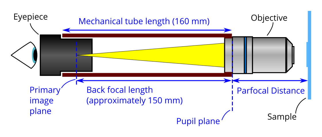
Many common objectives are designed for mechanical tube length of 160 mm, and have a parfocal distance of 45 mm (35 mm is also available). Some more expensive objectives are designed to focus at infinity, and require an extra lens to form an image (more on this later). Objectives that have a finite mechanical tube length are called finite conjugate objectives, those that focus at infinity are called infinite conjugate objectives. As standard we use a finite conjugate objective in the OpenFlexure microscope. However, the microscope can be adapted for infinite conjugate objectives.
Light exits the objective at the exit pupil, which lies on the pupil plane approximately in line with the shoulder. An image is formed on the primary imaging plane of the eyepiece, where it is viewed by the user. When building the OpenFlexure Microscope we use a camera sensor (a camera with the lens removed) instead of an eyepiece. We need the plane of the camera sensor to be where the primary image plane of the eyepiece would be, this is set by the back focal length of the objective. The back focal length is about 10 mm less than the mechanical tube length. To reduce the size of the microscope and to increase the field of view we use a extra lens called a tube lens.
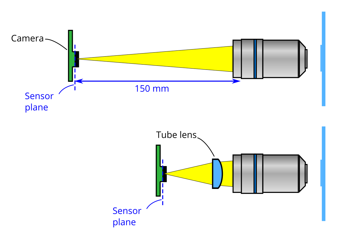
The position of the camera now depends on both the position of this tube lens, and the focal distance of the lens.
Using a tube lens also allows us to use an infinite conjugate objective, however we need a different separation between the lens and the sensor plane. Light exiting an infinite conjugate objective is collimated (or is said to form an image at infinity). As such, a tube lens is always needed to form an image inside a microscope if an infinite conjugate objective.
Calculating of lens-sensor distance
Starting again the thin lens equation
where:
- is the distance from the tube lens to the sensor
- is the distance from the tube lens to the primary imaging plane of the objective, i.e. where the image would be formed if there was no tube lens. (Note: This is negative as it is on the same side of the lens as image plane)
- is the focal length of the tube lens:
As we are now interested in we can rearrange to:
Calculation of desired tube lens
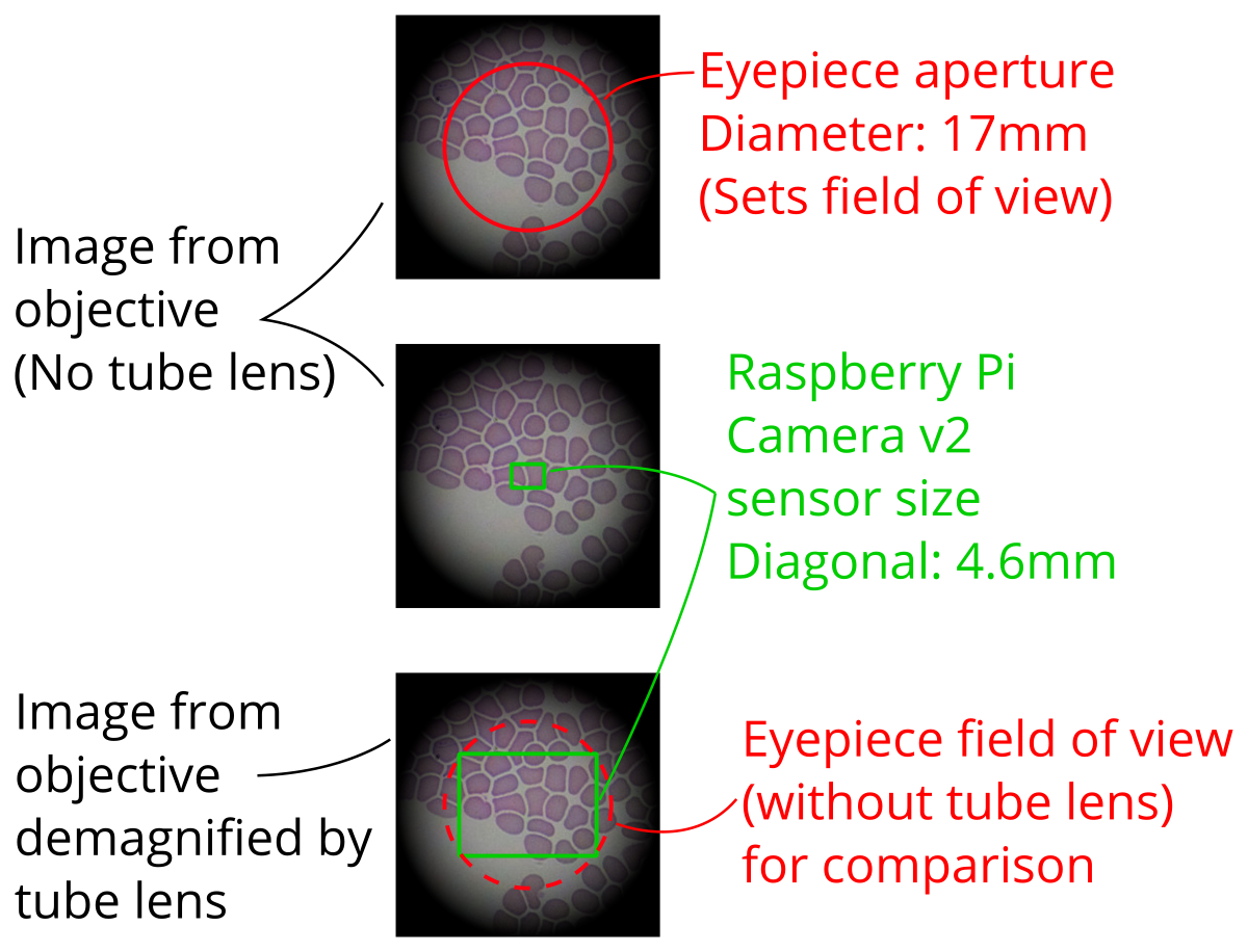
The tube lens will demagnify (shrink) the image on the sensor, this is useful as the sensor of the camera is smaller than a microscope eyepiece.
A traditional microscope will form an image that can be viewed with an eyepiece. The eyepiece will have an aperture at this image plane, this will set the field of view. This aperture size is called the field number (FN) and is quoted in millimeters. The field number can range from about 14-26 mm depending on the application. We assume 17 mm to be a standard field number. The sensor of most cameras is much smaller than this. We use a Raspberry Pi v2 camera sensor with a diagnoal of 4.6 mm. The desired magnification should match the field of view of the eyepiece to the field of view of the camera sensor:
We calculate the desired magnification as
In the case of the Raspberry Pi Camera v2, the diagonal sensor size is 4.6 mm so the desired magnification is 4.6/17 = 0.27.
The magnification, , is equal to
If we insert this the thin lens equation above we get can rearrange this to give
distance from the lens to the objective (set to 8.5 mm) minus the back focal length (150 mm). Therefore, for the Raspberry Pi Camera v2 the we calculate the optimal focal length for the tube lens as
We then choose 50 mm as the focal length as it is an easy to purchase focal length. This has a slight effect on the magnification. By rearranging the above we calculate the magnification for this lens as
For the Raspberry Pi Camera v2 and a 50 mm focal length tube lens
We can now calculate the effective field number of the diagonal of the Raspberry Pi Camera v2 sensor as
This falls well within the range of standard eyepiece field numbers (14-26 mm).
If you wish to use modify the microscope to use a different tube lens or a different camera sensor, then these calculations should be repeated for your setup.